Chapter 4: Comparison of Model-Free, SDM, LeMaster’s Approach, and Detectors

The following analysis was originally prepared for the 2023 Windischleuba NMR Summer School.

In the following, we will load a data set consisting of \(^{15}\)N relaxation data acquired for ubiquitin in solution, and analyze it using five methods: Spectral Density Mapping, LeMaster’s Approach, IMPACT, Detector Analysis (with and without removing tumbling), and Model-Free Analysis.

The data is taken from:

C. Charlier, S.N. Khan, T. Arquardsen, P. Pelupessy, V. Reiss, D. Sakellariou, G. Bodenhausen, F. Engelke, F. Ferrage. “Nanosecond time scale motions in proteins revealed by high-resolution NMR relaxometry.” J. Am. Chem. Soc. vol. 135, 18665-72 (2013).

(Thanks to Fabien for sharing!)

The methods used are:

Model-Free analysis

Lipari, G. & Szabo, A. Model-free approach to the interpretation of nuclear magnetic resonance relaxation in macromolecules. 1. Theory and range of validity. J. Am. Chem. Soc. vol. 104 4546–4559 (1982)

Spectral Density Mapping

Peng, J. & Wagner, G. Mapping of Spectral Density Functions Using Heteronuclear NMR Relaxation Measurements. J. Magn. Res. vol. 98 308–332 (1992)

LeMaster’s Approach

LeMaster, D. M. Larmor frequency selective model free analysis of protein NMR relaxation. J. Biomol. NMR vol. 6 366–374 (1995)

IMPACT

Khan, S.N., Charlier, C., Augustyniak, R., Salvi, N., Dejean, V., Bodenhausen, G., Lequin, O., Pelupessy, P., Ferrage, F. Distribution of Pico- and Nanosecond Motions in Disordered Proteins from Nuclear Spin Relaxation. Biophys. J. vol. 109 988-99 (2015)

Detector Analysis

Smith, A. A., Ernst, M. & Meier, B. H. Optimized ‘detectors’ for dynamics analysis in solid-state NMR. J. Chem. Phys. vol. 148 045104 (2018)

Smith, A. A., Ernst, M., Meier, B. H. & Ferrage, F. Reducing bias in the analysis of solution-state NMR data with dynamics detectors. J. Chem. Phys. vol. 151 034102 (2019)

Setup

# SETUP pyDR
import os
os.chdir('../..')

# Imports, misc. setup
import pyDR
import matplotlib.pyplot as plt
import numpy as np

from scipy.optimize import lsq_linear as lstsq

pyDR.Defaults['zrange'] = [-13,-6,200]

import matplotlib
matplotlib.rcParams.update({'font.size':16})

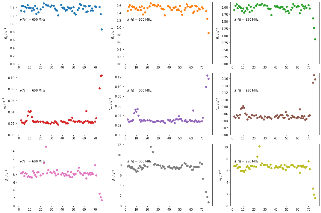
Load and plot the data

Note we split the data by field because Spectral Density Mapping (SDM) and LeMaster’s approach only operate on data from one field.

#Load the data
data=pyDR.IO.readNMR('https://raw.githubusercontent.com/alsinmr/pyDR_tutorial/main/data/ubi_soln.txt')
data.info['med_val']=None

#Split into one-field data for SDM, LeMaster's approach
data600=data.__copy__()
data600.del_exp([0,1,3,4,6,7])
data800=data.__copy__()
data800.del_exp([0,2,3,5,6,8])
data950=data.__copy__()
data950.del_exp([1,2,4,5,7,8])

cm=plt.get_cmap('tab10')  #Color map (use for selecting colors)

fig,ax=plt.subplots(3,3)
fig.set_size_inches([15,10])
ax=ax.flatten()
k=0
for exp in [r'$R_1$',r'$\Gamma_{HN}$',r'$R_2$']:
    for field in [600,800,950]:
        ax[k].scatter(data.label,data.R[:,k],color=cm(k))
        ax[k].set_ylabel(exp+r' / s$^{-1}$')
        ax[k].set_ylim([0,ax[k].get_ylim()[1]])
        ax[k].text(1,ax[k].get_ylim()[1]*.7,r'$\nu(^1H)$ = '+str(field)+' MHz')
        k+=1
fig.tight_layout()

Warning: Assigned sensitivity object did not equal detector sensitivities. Re-defining detector object

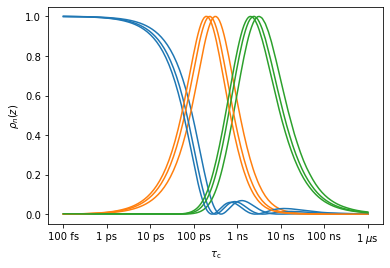
Spectral Density Mapping

Spectral density mapping is achieved simply by calculating linear combinations of the experimental relaxation rate constants at one field, as follows:

\[\begin{split} \begin{eqnarray} J(0)&=&\frac{R_2-R_1/2-0.454\sigma_\mathrm{IS}}{\delta_\mathrm{IS}^2/2+2(\Delta\sigma_\mathrm{I}\omega_\mathrm{I})^2} \\ J(\omega_\mathrm{I})&=&\frac{R_1-1.249\sigma_\mathrm{IS}}{3(\delta_\mathrm{IS}/4)^2+(\Delta\sigma_\mathrm{I}\omega_\mathrm{I})^2/3} \\ J(0.870\omega_\mathrm{S})&=&\frac{16\sigma_\mathrm{IS}}{5\delta_\mathrm{IS}^2} \end{eqnarray} \end{split}\]

This results in the following windows, resulting from the spectral density calculated for a given value of \(\tau_c\) and \((1–S^2)=1\).

\[ \begin{equation} J(\omega,\tau_c)=\frac25\frac{\tau_c}{1+(\omega\tau_c)^2} \end{equation} \]

fig,ax=plt.subplots(1,3)
fig.set_size_inches([12,4])
J=lambda omega,tc:2/5*tc/(1+(omega*tc)**2)
titles=(r'$J(0)$',r'$J(\omega_{N})$',r'$J(0.870*\omega_{H})$')

v0H0=[600,800,950]
rat=pyDR.tools.NucInfo('15N')/pyDR.tools.NucInfo('1H') #Ratio of 15N to 1H Larmor frequency
tc=np.logspace(-12,-7,200)
for v0H,a in zip(v0H0,ax):
    a.semilogx(tc,J(0,tc))
    a.semilogx(tc,J(v0H*2*np.pi*rat*1e6,tc))
    a.semilogx(tc,J(v0H*2*np.pi*0.87*1e6,tc))
    if a.is_first_col():
        a.set_ylabel(r'$J(\omega)$ / s')
    else:
        a.set_yticklabels('')
    a.set_ylim([0,0.75e-9])
    a.set_xlabel(r'$\tau_c$')
    a.set_title(r'$\nu_0(^1$H)'+f' = {v0H} MHz')
ax[0].legend(titles)
fig.tight_layout()

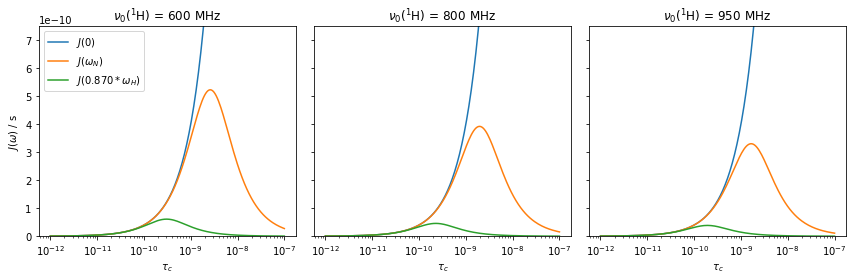
print(f'From the rotational correlation time, 4.84e-9 s, we estimate J(0) should be slightly less than {2/5*4.84e-9} s')

From the rotational correlation time, 4.84e-9 s, we estimate J(0) should be slightly less than 1.936e-09 s

Plot the SDM results

fig,ax=plt.subplots(3,3)
fig.set_size_inches([14,10])

titles=(r'$J(0)$',r'$J(\omega_{N})$',r'$J(0.870*\omega_{H})$')

delta=22954*2*np.pi/2  #rad/s
Del_sig=172   #ppm

J0=list()
JomegaI=list()
Jp87omegaS=list()
for v0H,d,a in zip(v0H0,[data600,data800,data950],ax.T):
    #data in d has residues down the columns and R1,NOE,R2 across the rows
    DSOmega=Del_sig*v0H*rat*2*np.pi   #DeltaSigma_I*omega_I  (rad/s)
    dd=delta
    c=Del_sig*v0H*rat*2*np.pi/np.sqrt(3)
    
    J0.append((d.R[:,2]-d.R[:,0]/2-0.454*d.R[:,1])/(3*dd**2+4*c**2)*6)
    JomegaI.append((d.R[:,0]-1.249*d.R[:,1])/(3*dd**2/4+c**2))
    Jp87omegaS.append(4*d.R[:,1]/(5*dd**2))
    
    for k,(J,title) in enumerate(zip([Jp87omegaS[-1],JomegaI[-1],J0[-1]],titles[::-1])):
        a[k].scatter(d.label,J*1e9,color=cm(k))
        a[k].set_ylabel(title+' / 1e-9 s')
        if a[k].is_first_row():
            a[k].set_title(r'$\nu_0(^1H)$'+f' = {v0H} MHz')
    a[0].set_ylim([0,.03])
    a[1].set_ylim([0,.5])
    a[2].set_ylim([0,3])
fig.tight_layout()

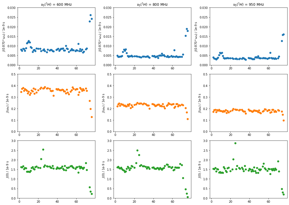
Note that the spike in \(J(0)\) at residues 21-23 is likely due to chemical exchange, and is not due to reorientional dynamics.

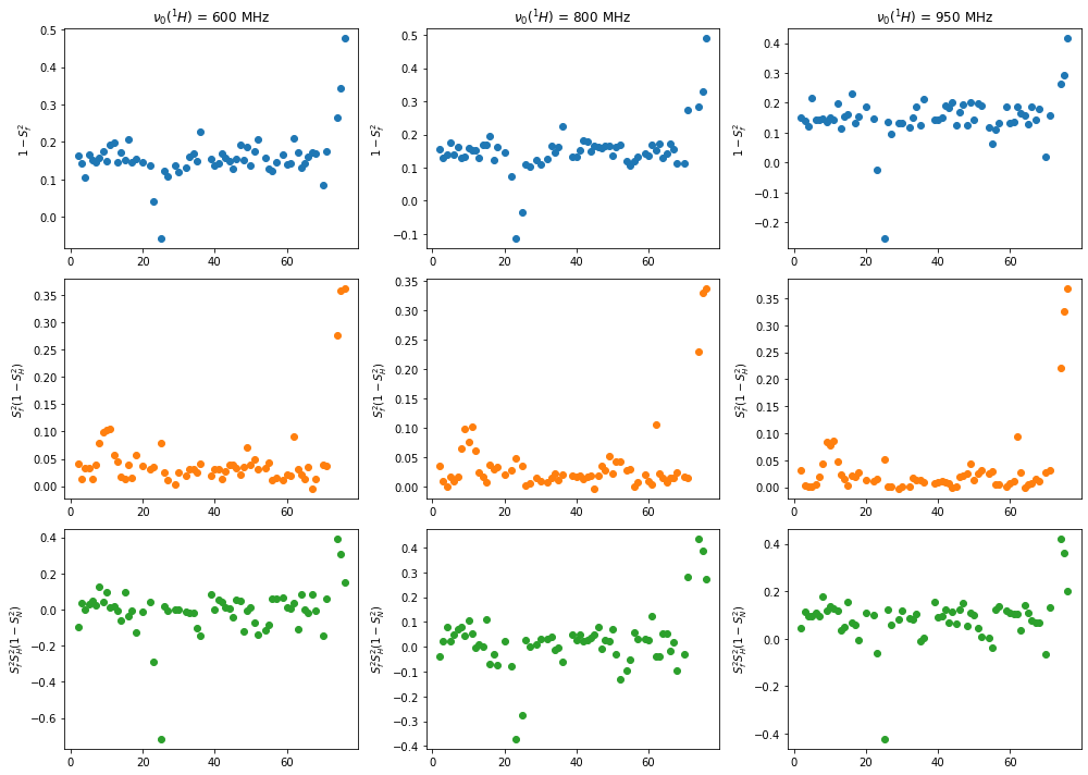
LeMaster’s Approach

LeMaster uses a similar approach, but fits the data to a model spectral density, which allows one to separate out the influence of tumbling from the internal motion.

\[\begin{split} \begin{eqnarray} J(\omega)= &\frac25&\left[\frac{\tau_M}{1+(\omega\tau_M)^2}+(1-S_f^2)\left(-\frac{\tau_M}{1+(\omega\tau_M)^2}\right)+\right.\\ &&\left.S_f^2(1-S_H^2)\left(\frac{\tau_H}{1+(\omega\tau_H)^2}-\frac{\tau_M}{1+(\omega\tau_M)^2}\right)+S_f^2S_H^2(1-S_N^2)\left(\frac{\tau_N}{1+(\omega\tau_N)^2}-\frac{\tau_M}{1+(\omega\tau_M)^2}\right)\right] \end{eqnarray} \end{split}\]

with

\[\begin{split} \begin{eqnarray} \tau_H&=&(\omega_H+\omega_N)^{-1} \\ \tau_N&=&|\omega_N|^{-1} \end{eqnarray} \end{split}\]

Then, the parameters \(1-S_f^2\), \(S_f^2(1-S_H^2)\), and \(S_f^2S_H^2(1-S_N^2)\) can be used to fit the relaxation rate constants or the spectral densities directly in a linear fit.

We’ll use the results from the SDM, rather than trying to do the fits directly from the raw data.

We know from previously published results (Charlier et al.) that the rotational correlation time, \(\tau_M\), is 4.84 ns

Plot results from LeMaster’s Approach

fig,ax=plt.subplots(3,3)
fig.set_size_inches([14,10])

tM=4.84e-9  #Rotation diffusion correlation time / s

titles=(r'$1-S_f^2$',r'$S_f^2(1-S_H^2)$',r'$S_f^2S_H^2(1-S_N^2)$')

for v0H,J00,JomegaI0,Jp87omegaS0,a in zip(v0H0,J0,JomegaI,Jp87omegaS,ax.T):
    tH=1/(v0H*2*np.pi*1e6+v0H*rat*2*np.pi*1e6)
    tN=1/np.abs(v0H*rat*2*np.pi*1e6)
        
    omega0=[0,-v0H*rat*2*np.pi*1e6,0.87*v0H*2*np.pi*1e6]  #Frequencies sampled by SDM in rad/s
    
    offset=np.zeros(3)  #This is the offset term, 2/5*tM/(1+omega*tM)
    M=np.zeros((3,3))
    for k,omega in enumerate(omega0):
        offset[k]=2/5*tM/(1+(omega*tM)**2)
        #M@[(1-Sf2),Sf2*(1-SH2),Sf2*SH2*(1-SN2)] = [J0,JomegaN,0.87*JomegaH]
        M[k]=[-2/5*tM/(1+(omega*tM)**2),2/5*(tH/(1+(omega*tH)**2)-tM/(1+(omega*tM)**2)),
              2/5*(tN/(1+(omega*tN)**2)-tM/(1+(omega*tM)**2))]
    
    A0=np.linalg.pinv(M)@(np.array([J00,JomegaI0,Jp87omegaS0]).T-offset).T
#     A0=np.array([lsq(M,b)['x'] for b in np.array([J00,JomegaI0,Jp87omegaS0]).T-offset]).T
    
    for k,(A,title) in enumerate(zip(A0,titles)):
        a[k].scatter(d.label,A,color=cm(k))
        a[k].set_ylabel(title)
        if a[k].is_first_row():
            a[k].set_title(r'$\nu_0(^1H)$'+f' = {v0H} MHz')
fig.tight_layout()
       

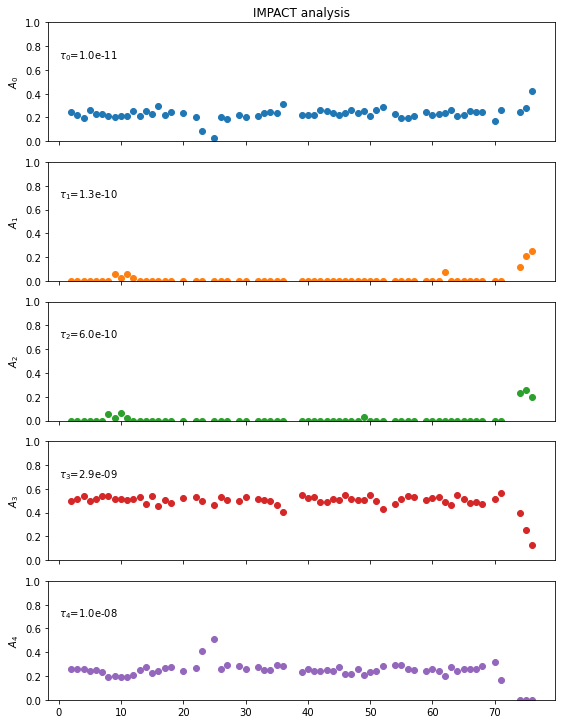
IMPACT Analysis of full data set

IMPACT assumes a correlation function which is a sum of several correlation times, where the sum of weights for the terms is 1. We will assume four correlation times here, such that

\[\begin{split} \begin{eqnarray} C(t)&=&\frac25\sum\limits_{i=1}^4{A_ie^{-t/\tau_i}} \\ 1&=&\sum\limits_{i=1}^4{A_i} \\ 0&\le&A_i\le1 \end{eqnarray} \end{split}\]

Plot IMPACT amplitudes

#I cheated a little bit here...
#I took the correlation times from the detector analysis below for the middle 3 values
#And then manually optimized the last and put the first to just a short correlation time
tau=10**np.array([-11,-9.9002036,-9.2239323,-8.5449795,-8]) #Array of correlation times
J=np.array([*J0,*JomegaI,*Jp87omegaS]) #Collect all spectra densities
norm=J.mean(1)  #Use for reweighting
omega=np.array([0,0,0,*(-rat*np.array(v0H0)),*(0.87*np.array(v0H0))])*1e6*2*np.pi

q=10

M=np.zeros([10,len(tau)])
for k,tau0 in enumerate(tau):
    M[:-1,k]=2/5*tau0/(1+(omega*tau0)**2)/norm
    M[-1,k]=q  #We'll use this position to enforce the sum of the Ai to 1

A=np.zeros([len(tau),J.shape[1]])
Jc=np.zeros(J.shape)
for k,X in enumerate(J.T):
    target=np.array([*(X/norm),q])
    out=lstsq(M,target,bounds=(0,1))
    A[:,k]=out['x']
    Jc[:,k]=(M@A[:,k])[:-1]*norm

fig,ax=plt.subplots(len(tau),1)
fig.set_size_inches([8,10])
for k,(a,A0) in enumerate(zip(ax,A)):
    a.scatter(data.label,A0,color=cm(k))
    a.set_ylim([0,1])
    a.set_ylabel(r'$A_{'+str(k)+r'}$')
    a.text(0,.7,r'$\tau_{'+str(k)+'}$'+f'={tau[k]:.1e}')
    if not(a.is_last_row()):
        a.set_xticklabels('')
fig.tight_layout()
ax[0].set_title('IMPACT analysis')

Text(0.5, 1.0, 'IMPACT analysis')

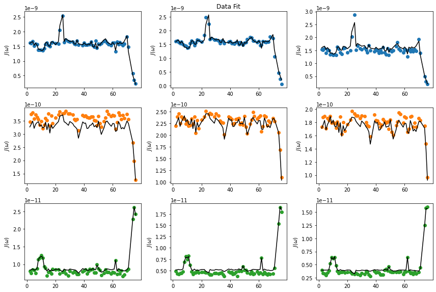
Plot data fit resulting from IMPACT analysis

fig,ax=plt.subplots(3,3)
fig.set_size_inches([12,8])
for k,(a,X,Xc) in enumerate(zip(ax.flatten(),J,Jc)):
    a.scatter(data.label,X,color=cm(k//3))
    a.plot(data.label,Xc,color='black')
    a.set_ylabel(r'$J(\omega)$')
fig.tight_layout()
ax[0,1].set_title('Data Fit')

Text(0.5, 1.0, 'Data Fit')

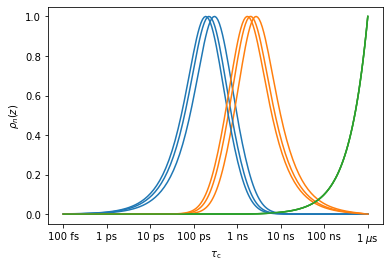
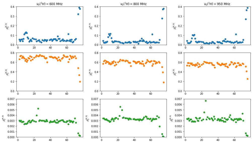
One-field detector analysis, first without removing tumbling

Detector analysis can be performed on the total motion, which means for solution-state data, the overall tumbling is included in the detector responses. We do this analysis first.

ax_sens=plt.subplots()[1]
fig,ax=plt.subplots(3,3)
fig.set_size_inches([14,8])
for k,(d,v0H,a) in enumerate(zip([data600,data800,data950],v0H0,ax.T)):
    #When loaded, a "solution-state" sensitivity is loaded, and includes tumbling influence
    #For the initial analysis, we replace this with a sensitivity that does not consider tumbling
    d.sens=pyDR.Sens.NMR(info=d.sens.info)
    d.detect.r_auto(3)
    fit=d.fit(bounds=True)
    fit.sens.plot_rhoz(ax=ax_sens,color=[cm(m) for m in range(3)])
    for m in range(3):
        a[m].scatter(fit.label,fit.R[:,m],color=cm(m))
        a[m].set_ylabel(r'$\rho_'+str(m)+r'^{(\theta,S)}$')
    a[0].set_ylim([0,.4])
    a[1].set_ylim([0,.8])
    a[2].set_ylim([0,.007])
    a[0].set_title(r'$\nu_0(^1H) = $'+f'{v0H} MHz')
fig.tight_layout()

Warning: Assigned sensitivity object did not equal detector sensitivities. Re-defining detector object
Warning: Assigned sensitivity object did not equal detector sensitivities. Re-defining detector object
Warning: Assigned sensitivity object did not equal detector sensitivities. Re-defining detector object

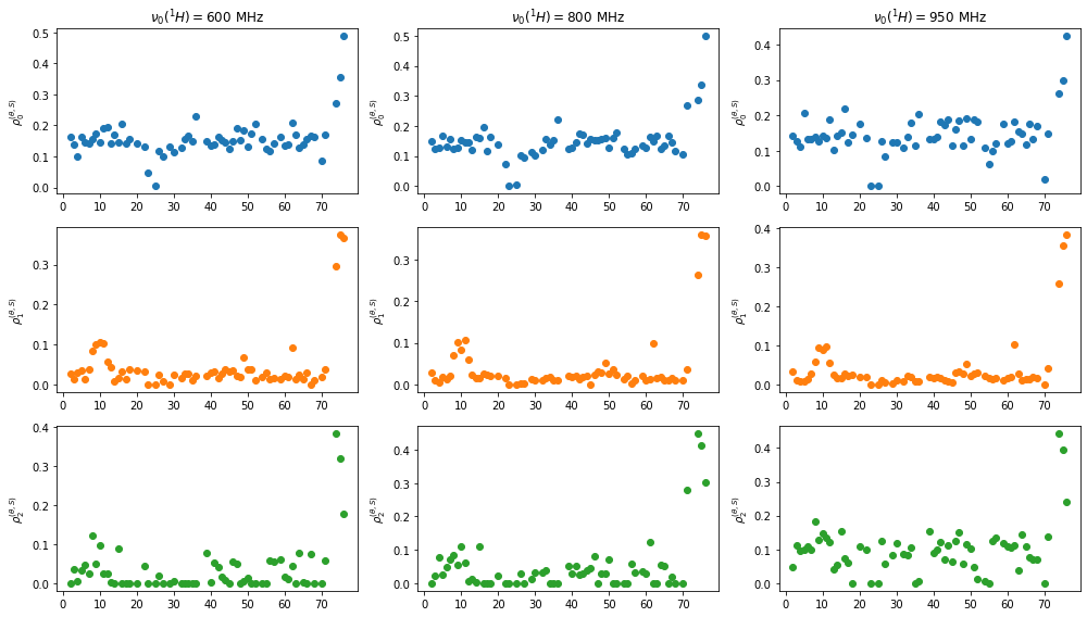
One-field detector analysis, including removing tumbling

We may also factor out isotropic tumbling, which is the case for sufficiently spherical molecules, so that detector responses represent only the internal motion. Note that this has a profound effect on the positioning of the detector windows, as discussed here.

ax_sens=plt.subplots()[1]
fig,ax=plt.subplots(3,3)
fig.set_size_inches([14,8])
for k,(d,v0H,a) in enumerate(zip([data600,data800,data950],v0H0,ax.T)):
    #When loaded, a "solution-state" sensitivity is loaded, and includes tumbling influence
    #For the initial analysis, we replace this with a sensitivity that does not consider tumbling
    d.sens=pyDR.Sens.SolnNMR(info=d.sens.info)
    d.detect.r_auto(3)
    fit=d.fit(bounds=True)
    fit.sens.plot_rhoz(ax=ax_sens,color=[cm(m) for m in range(3)])
    for m in range(3):
        a[m].scatter(fit.label,fit.R[:,m],color=cm(m))
        a[m].set_ylabel(r'$\rho_'+str(m)+r'^{(\theta,S)}$')
    a[0].set_title(r'$\nu_0(^1H) = $'+f'{v0H} MHz')
fig.tight_layout()

Warning: Assigned sensitivity object did not equal detector sensitivities. Re-defining detector object
Warning: Assigned sensitivity object did not equal detector sensitivities. Re-defining detector object
Warning: Assigned sensitivity object did not equal detector sensitivities. Re-defining detector object

Detector Analysis of full data set without removing tumbling

data.sens=pyDR.Sens.NMR(tc=np.logspace(-12,-7.9,200),info=data.sens.info)
data.S2=np.zeros(data.R.shape[0])
data.S2std=np.ones(data.R.shape[0])*.01
data.detect.r_auto(4)
fit=data.fit()
plt_obj=fit.plot(style='scatter')
plt_obj.fig.set_size_inches([7,12])
for a in plt_obj.ax[:-1]:a.set_ylim([0,1])
plt_obj.show_tc()

Warning: Assigned sensitivity object did not equal detector sensitivities. Re-defining detector object

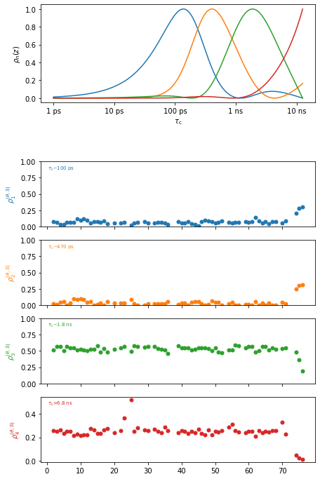
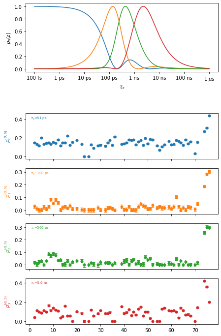
Detector Analysis of full data set including removing tumbling

zmax=[-14,*fit.info['zmax'][:-1]]
data.sens=pyDR.Sens.SolnNMR(info=data.sens.info)
data.detect.r_auto(4)
fit=data.fit()
plt_obj=fit.plot(style='scatter',errorbars=True)
plt_obj.fig.set_size_inches([7,12])
plt_obj.show_tc()

Warning: Assigned sensitivity object did not equal detector sensitivities. Re-defining detector object

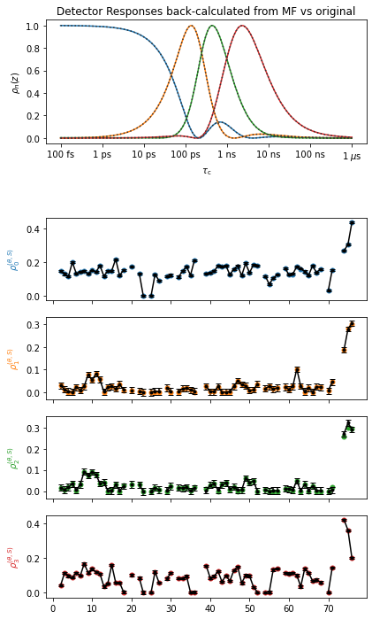
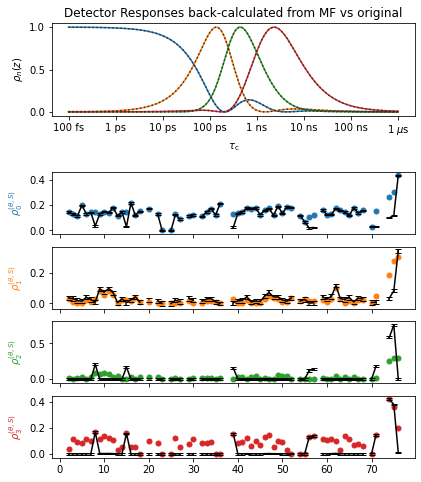
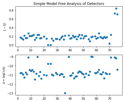
Model Free Analysis

In this analysis, we fit the internal motion of ubiquitin to a single correlation time, i.e. via the simple model free approach. Note that this is actually easier done to the results of the detector analysis rather than to the raw NMR data.

from pyDR.Fitting.fit import model_free
z,A,error,dfit=model_free(fit,nz=1)

plt_obj=fit.plot(style='scatter')
plt_obj.append_data(dfit)
plt_obj.ax_sens.set_title('Detector Responses back-calculated from MF vs original')
plt_obj.fig.set_size_inches([6.5,8])

fig,ax=plt.subplots(2,1)
fig.set_size_inches([6,5])
ax[0].scatter(fit.label,A[0],color=cm(0))
ax[0].set_ylabel(r'$1-S_f^2$')
ax[1].scatter(fit.label,z[0],color=cm(0))
ax[1].set_ylabel(r'$z_f=\log(\tau_f$/s)')
ax[0].set_title('Simple Model-Free Analysis of Detectors')
fig.tight_layout()

1 of 1 iterations

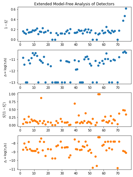
Extended Model-free analysis of full data set

Finally, we use an extended model free analyis. Note that for extended model free analysis, one would typically do a residue-specific model selection, where the number of free parameters is variable (correlation times, order parameters). We do not do that here, always fitting to 2 correlation times and two amplitudes (resulting in slightly different plots than found in Charlier et al.).

Plot the Model Free parameters

from pyDR.Fitting.fit import model_free
z,A,error,dfit=model_free(fit,nz=2)

fig,ax=plt.subplots(4,1)
fig.set_size_inches([6,8])
ax[0].scatter(fit.label,A[0],color=cm(0))
ax[0].set_ylabel(r'$1-S_f^2$')
ax[1].scatter(fit.label,z[0],color=cm(0))
ax[1].set_ylabel(r'$z_f=\log(\tau_f$/s)')
ax[2].scatter(fit.label,A[1],color=cm(1))
ax[2].set_ylabel(r'$S_f^2(1-S_s^2)$')
ax[3].scatter(fit.label,z[1],color=cm(1))
ax[3].set_ylabel(r'$z_s=\log(\tau_s$/s)')
ax[0].set_title('Extended Model-Free Analysis of Detectors')
fig.tight_layout()

1 of 4 iterations
2 of 4 iterations
3 of 4 iterations
4 of 4 iterations

Plot the fit of the detector responses

plt_obj=fit.plot(style='scatter')
plt_obj.append_data(dfit,marker='o',markersize=3)
plt_obj.ax_sens.set_title('Detector Responses back-calculated from MF vs original')
plt_obj.fig.set_size_inches([6.5,12])