REDOR#
![]()
Rotational-Echo DOuble Resonance NMR (REDOR\(^1\)) is an important technique for dynamics measurements,\(^{2,3}\) where applying REDOR to one-bond dipole couplings allows one to compare the known size of the rigid dipole coupling, to its measured size, which is reduced due to dynamics. This yields the order parameter, \(S\), according to
We do not obtain the sign of the dipole coupling from REDOR, so we only get the absolute value of \(S\).
Here, we investigate how REDOR behaves as a function of correlation time.
Note, this was the topic of a recent paper by Aebischer et al.,\(^4\) where simulations were performed using Gamma\(^5\). We hope SLEEPY makes this type of simulation more accessible.
[1] T. Gullion, J. Schaefer. J. Magn. Reson., 1989, 196-200.
[2] V. Chevelkov, U. Fink. B. Reif. J. Am. Chem. Soc., 2009, 131, 14018-14022.
[3] P. Schanda, B.H. Meier, M. Ernst. J. Magn. Reson., 2011, 210, 246-259.
[4] K. Aebischer, L.M. Becker, P. Schanda, M. Ernst. Magn. Reson., 2024, 5, 69-86
[5] S.A. Smith, T.O. Levante, B.H. Meier, R.R. Ernst. J. Magn. Reson. A, 1994, 106, 75-105.
Setup#
import SLEEPY as sl
import numpy as np
import matplotlib.pyplot as plt
from time import time
Build the system#
We construct a system undergoing 3-site symmetric exchange, in order to obtain a residual dipole coupling without asymmetry (\(\eta\)=0). The sl.Tools.Setup3siteSym(...) function is used to create the three-site hopping motion out of the initial system, ex0.
ex0=sl.ExpSys(v0H=600,Nucs=['15N','1H'],vr=60000,pwdavg=sl.PowderAvg('bcr20'),n_gamma=30)
# After varying the powder average and n_gamma
# a beta-average and 30 gamma angles were determined to be sufficient
delta=sl.Tools.dipole_coupling(.102,'15N','1H')
phi=35*np.pi/180

ex0.set_inter('dipole',i0=0,i1=1,delta=delta)
L=sl.Tools.Setup3siteSym(ex0,tc=1e-9,phi=phi)
Generate and plot pulse sequences#
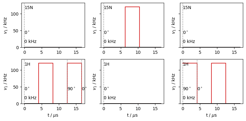
We break the REDOR sequence up into three sequences (L.Sequence()), a first half (first) with \(^1\)H \(\pi\)-pulses coming in the middle and end of the rotor period, a middle sequence (center) with a \(^{15}\)N \(\pi\)-pulse to refocus the \(^{15}\)N chemical shift, and a second half (second) with \(^1\)H \(\pi\)-pulses coming at the beginning and middle of the rotor period.
v1=120e3 #100 kHz pulse
tp=1/v1/2 #pi/2 pulse length

t=[0,L.taur/2-tp,L.taur/2,L.taur-tp,L.taur]
first=L.Sequence().add_channel('1H',t=t,v1=[0,v1,0,v1],phase=[0,0,0,np.pi/2,0])
t=[0,tp,L.taur/2,L.taur/2+tp,L.taur]
second=L.Sequence().add_channel('1H',t=t,v1=[v1,0,v1,0],phase=[np.pi/2,0,0,0,0])
center=L.Sequence().add_channel('15N',t=[0,L.taur/2-tp/2,L.taur/2+tp/2,L.taur],
                               v1=[0,v1,0])

rho=sl.Rho('15Nx','15Nx')
We plot the three sequences below.
fig,ax=plt.subplots(2,3,figsize=[8,4],sharey=True)
first.plot(ax=ax.T[0])
center.plot(ax=ax.T[1])
second.plot(ax=ax.T[2])
fig.tight_layout()
Propagation#
We first generate a propagator for each of the three sequences (Ucenter,Ufirst,Usecond). Then below, we create two propagators for the first (U1) and second half (U2) of the sequence which are increased in length by one rotor period at every step of the rotor period.
Ucenter=center.U()
Ufirst=first.U()
Usecond=second.U()
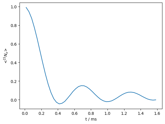
At each step below, the density matrix (rho), is set back to the initial time via rho.reset(), and then multiplied with propagators for the first half (U1), the center (Ucenter), and for the second half (U2), where U1 and U2 are each increased by one rotor period at every step. (U2*Ucenter*U1*rho)() propagates rho with the full REDOR sequence, followed by detection (don’t forget the parenthesis!).
rho=sl.Rho('15Nx','15Nx')
U1=L.Ueye()
U2=L.Ueye()

t0=time()
for k in range(48):
    rho.reset()
    (U2*Ucenter*U1*rho)()
    U1=Ufirst*U1
    U2=Usecond*U2
print(time()-t0)
19.125797986984253
_=rho.plot()
Reducible sequence#
The above sequence is computationally expensive, requiring a basis set of 48 elements. If we consider that we’re mainly interested in the \(S^+\) operator of the \(^{15}\)N spin, then its worth noting that the \(^{15}\)N \(\pi\)-pulse in the middle of the sequence converts \(S^+\) into \(S^-\), \(S^\alpha\), and \(S^\beta\), so that if we could get rid of it, we could use a basis set 1/4 as big (12 elements). Since there is no \(^{15}\)N chemical shift included in our simulation, we can switch the channel of the middle pulse to \(^1\)H. An alternative approach would be to use a \(\delta\)-pulse on \(^{15}\)N, although the basis set would then only be reduced to 24 elements, since \(S^+\) would still be converted to \(S^-\)
centerH=L.Sequence().add_channel('1H',t=[0,L.taur/2-tp/2,L.taur/2+tp/2,L.taur],v1=[0,v1,0])

rho=sl.Rho('15Np','15Nx')

rho,f,s,c,Ueye=rho.ReducedSetup(first,second,centerH,L.Ueye())
State-space reduction: 48->12
Ufirst=f.U()
Usecond=s.U()
Ucenter=c.U()
U1=Ueye
U2=Ueye

t0=time()
for k in range(48):
    rho.reset()
    (U2*Ucenter*U1*rho)()
    U1=Ufirst*U1
    U2=Usecond*U2
print(time()-t0)
9.653581857681274
_=rho.plot()

We see that the reduced sequence yields the same results as before, but with matrices only 1/16 as big as the previous calculation.
Sweep the correlation time#
We now re-run the above setup, but while varying the correlation time to observe the transition between having a fully averaged dipole coupling and having the rigid-limit coupling.
rho_list=[]
legend=[]
t0=time()
for tc in np.logspace(-6,-3,8):
    L.kex=sl.Tools.nSite_sym(n=3,tc=tc)

    rho_list.append(rho.copy_reduced())

    Ufirst=f.U()
    Usecond=s.U()
    Ucenter=c.U()

    U1=Ueye
    U2=Ueye

    for k in range(28):
        rho_list[-1].reset()
        (U2*Ucenter*U1*rho_list[-1])()

        U1=Ufirst*U1
        U2=Usecond*U2

    legend.append(fr'$\log_{{10}}(\tau_c)$ = {np.log10(tc):.1f}')
    print(f'log10(tc /s) = {np.log10(tc):.1f}, {time()-t0:.0f} seconds elapsed')
log10(tc /s) = -6.0, 8 seconds elapsed
log10(tc /s) = -5.6, 17 seconds elapsed
log10(tc /s) = -5.1, 25 seconds elapsed
log10(tc /s) = -4.7, 34 seconds elapsed
log10(tc /s) = -4.3, 42 seconds elapsed
log10(tc /s) = -3.9, 50 seconds elapsed
log10(tc /s) = -3.4, 58 seconds elapsed
log10(tc /s) = -3.0, 66 seconds elapsed
fig,ax=plt.subplots(2,4,figsize=[9,4.5])
ax=ax.flatten()
for a,l,r in zip(ax,legend,rho_list):
    r.plot(ax=a)
    a.set_title(l)
    if not(a.is_first_col()):
        a.set_ylabel('')
        a.set_yticklabels([])
    if not(a.is_last_row()):
        a.set_xlabel('')
        a.set_xticklabels([])
fig.tight_layout()
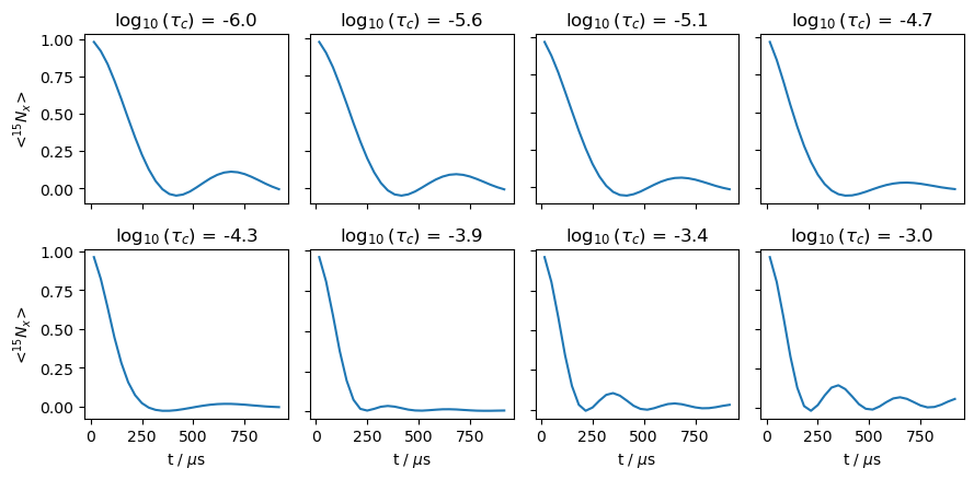
We observe above that when the correlation time is shorter than about 100 \(\mu\)s, we see the fully averaged coupling, and when the correlation time is longer than about 1 ms, we obtain the rigid-limit value. In between, oscillations are damped due to dynamics being on the timescale of the coupling.