Short Examples

The following notebook shows some simulations that can be done in just a few lines of code. These are intended to familiarize you with the basics of setting up SLEEPY simulations.

Setup

import SLEEPY as sl
import numpy as np

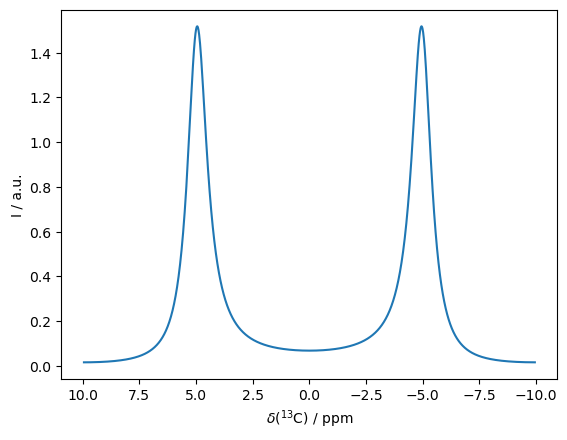
1D Spectrum in Exchange

Two peaks, separated by 10 ppm, with a correlation time of exchange of 1 ms.

ex0=sl.ExpSys(v0H=600,Nucs='13C')
ex1=ex0.copy()
ex0.set_inter('CS',i=0,ppm=5)
ex1.set_inter('CS',i=0,ppm=-5)

L=sl.Liouvillian(ex0,ex1,kex=sl.Tools.twoSite_kex(tc=1e-3))
seq=L.Sequence(Dt=1/3000)  #1/(2*10 ppm*150 MHz)

rho=sl.Rho('13Cx','13Cp')
rho.DetProp(seq,n=4096)
_=rho.plot(FT=True,axis='ppm')

State-space reduction: 8->2

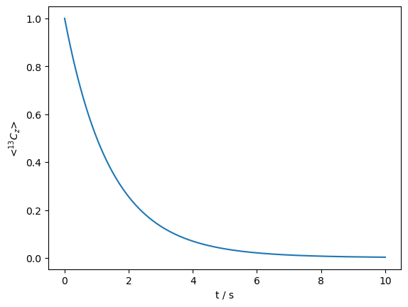
\(T_1\) relaxation in solid-state NMR

\(^{13}\)C \(T_1\) relaxation in solid-state NMR, due to a 30\(^\circ\) reorientation of the H–C dipole coupling, occuring with a correlation time of 1 ns.

ex0=sl.ExpSys(v0H=600,Nucs=['13C','1H'],vr=10000,LF=True)  #T1 occurs only due to terms in the lab frame
ex1=ex0.copy()
ex0.set_inter('dipole',i0=0,i1=1,delta=44000)
ex1.set_inter('dipole',i0=0,i1=1,delta=44000,euler=[0,30*np.pi/180,0])

L=sl.Liouvillian(ex0,ex1,kex=sl.Tools.twoSite_kex(tc=1e-9))
seq=L.Sequence() #Defaults to 1 rotor period

rho=sl.Rho('13Cz','13Cz')
rho.DetProp(seq,n=10000*10) #10 seconds
_=rho.plot(axis='s')

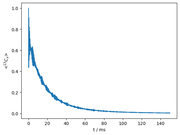
\(T_{1\rho}\) relaxation

\(^{13}\)C \(T_{1\rho}\) relaxation in solid-state NMR, due to a 30\(^\circ\) reorientation of the H–C dipole coupling, occuring with a correlation time of 100 ns.

ex0=sl.ExpSys(v0H=600,Nucs=['13C','1H'],vr=10000)
ex1=ex0.copy()
ex0.set_inter('dipole',i0=0,i1=1,delta=44000)
ex1.set_inter('dipole',i0=0,i1=1,delta=44000,euler_d=[0,30,0])

L=sl.Liouvillian(ex0,ex1,kex=sl.Tools.twoSite_kex(tc=1e-7))
seq=L.Sequence().add_channel('13C',v1=25000) #Defaults to 1 rotor period

rho=sl.Rho('13Cx','13Cx')
rho.DetProp(seq,n=1500) #100 ms
_=rho.plot()

State-space reduction: 32->16

Chemical Exchange Saturation Transfer

CEST is useful when a system has a major and minor population, the minor being invisible in the spectrum. However, applying a saturating field to the minor population will still be effective in saturating the major population, so that we may sweep the frequency of the saturating field to find the minor population’s resonance frequency.

In this simple example, we’ll just monitor the total z-magnetization, although in the real experiment we would integrate the peak with high population (also possible in SLEEPY, but requires additional steps to acquire the full direct dimension and integrate over the correct peak).

ex0=sl.ExpSys(v0H=600,Nucs='13C')
ex1=ex0.copy()
ex0.set_inter('CS',i=0,Hz=750)
ex1.set_inter('CS',i=0,Hz=-750)

L=sl.Liouvillian(ex0,ex1,kex=sl.Tools.twoSite_kex(tc=1e-1,p1=.95))  #5% population 2
L.add_relax('T1',i=0,T1=1)
L.add_relax('T2',i=0,T2=.1)
L.add_relax('recovery')
seq=L.Sequence(Dt=.5)  #1/(2*10 ppm*150 MHz)

rho=sl.Rho('13Cz','13Cz')
voff0=np.linspace(-1500,1500,101)

for voff in voff0:
    rho.reset()
    seq.add_channel('13C',v1=50,voff=voff)
    (seq*rho)()
ax=rho.plot()
ax.set_xticks(np.linspace(0,101,11))
ax.set_xticklabels(voff0[np.linspace(0,100,11).astype(int)]/1000)
_=ax.set_xlabel(r'$\nu_{off}$ / kHz')

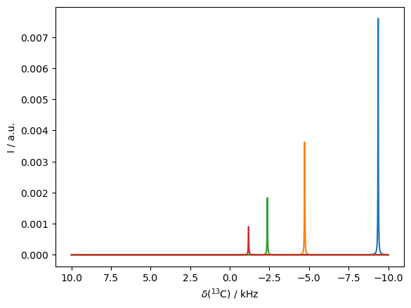
Contact shift

The contact shift comes from the hyperfine coupling between a fast-relaxing electron and a nucleus. While the fast relaxing electron averages the splitting, the peak itself shifts due to polarization of the electron.

We’ll run the simulation as a function of temperature, where lower temperatures yield a higher shift (and more signal). Note that realistically, we wouldn’t expect the electron relaxation times to remain fixed with the varying temperature.

ax=None
ex=sl.ExpSys(v0H=600,Nucs=['13C','e']).set_inter('hyperfine',i0=0,i1=1,Axx=1e5,Ayy=1e5,Azz=1e5)
for T in [50,100,200,400]:
    ex.T_K=T
    L=ex.Liouvillian()
    L.add_relax('T1',i=1,T1=1e-9)
    L.add_relax('T2',i=1,T2=1e-10)
    L.add_relax('recovery')

    seq=L.Sequence(Dt=5e-5)

    rho=sl.Rho('13Cx','13Cp')
    ax=rho.DetProp(seq,n=2048).plot(FT=True,ax=ax)

State-space reduction: 16->2
State-space reduction: 16->2
State-space reduction: 16->2
State-space reduction: 16->2

Spinning sidebands (one liner)

The last simulation is a little bit just for fun, but also to demonstrate some of the convenience of object-oriented programming in SLEEPY. We simulate \(^{13}\)C spinning sidebands resulting from chemical shift anisotropy. However, we set up the whole simulation in a single (broken) line of code and plot the result.

Compare to Herzfeld/Berger figure 2c.\(^1\)

[1] J. Herzfeld, A.E. Berger. J.Chem. Phys. 1980, 73, 6021-6030.

_=sl.Rho('31Px','31Pp').DetProp(
    sl.ExpSys(B0=6.9009,Nucs='31P',vr=2060).set_inter('CSA',i=0,delta=-104,eta=.56).\
    Liouvillian().Sequence(),
    n=4096,n_per_seq=20).plot(FT=True,axis='kHz',apodize=True)

State-space reduction: 4->1
Prop: 20 steps per every 1 rotor period